Descriptive Statistics Box

Take a look at this box. You can see each condition name in left most column. If you have given your conditions meaningful names, you should know exactly which conditions these names represent. You can find out the number of participants, the mean and standard deviation for each condition by reading across each of the three condition rows.

Example

In this Descriptive Statistics box, the mean for the caffeine condition is 5.40. The mean the mean for the juice condition is 7.20 and the mean for the beer condition is 9.40. The standard deviation for the caffeine condition is 1.14, the standard deviation for the juice condition is 1.10 (when rounded) and the standard deviation for the beer condition is 1.14.  The number of participants in each condition (N) is 5.

Compare the Means

We use ANOVA to determine if the means are statistically different. But you don’t have to use ANOVA to find out some basic information about mean differences. Compare your means. Which one is the highest? Which is the lowest? If you were to find significant differences with your ANOVA, what do these directional differences in the means say about your results? In this example, the mean for the beer condition is 9.4 hours of sleep whereas the mean for the caffeine condition is 5.4 hours of sleep. The mean for the juice condition, 7.2, falls in between these two. So just eyeballing it, we can see that there are more hours slept in the beer condition when compare to the others. We need our ANOVA to determine if the differences between condition means are significant. We need ANOVA to make a conclusion about whether the IV (drink type) had an effect on the DV (number of hours slept). But looking at the means can give us a head start in interpretation.

Multivariate Tests Box

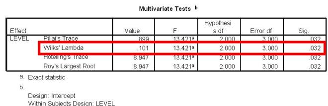
This is the next box you will look at. It contains info about the 1-Way Within Subjects ANOVA that you conducted. There are many different variations of this test. Most undergraduates use the “Wilks’ Lambda” variation. So, unless you are instructed otherwise, it is likely that you will want to read from only the Wilks’ Lambda row.

Sig value

Take a look at the Sig value, presented in the last column. Make sure you are reading from the Wilks’ Lamba row. This value will tell you if the three condition Means are statistically different. Often times, this value will be referred to as the p value. In this example, the Sig value in the Wilks’ Lamba row is 0.032.

If the Sig value is greater than 05…

You can conclude that there is no statistically significant difference between your three conditions. You can conclude that the differences between condition Means are likely due to chance and not likely due to the IV manipulation.

If the Sig value is less than or equal to .05…

You can conclude that there is a statistically significant difference between your three conditions. You can conclude that the differences between condition Means are not likely due to change and are probably due to the IV manipulation.

Our Example

The Sig. value in our example is 0.032. This value is less than .05. Because of this, we can conclude that there is a statistically significant difference between the mean hours of sleep between some or all of our conditions (caffeine, juice and beer).

The problem

The Sig value does not tell you which condition means are different. It could be that only the caffeine condition is significantly different than the juice condition in terms of hours of sleep. It could be that only the caffeine condition is significantly different than the beer condition. It could be that all conditions are significantly different from each other. The Sig value can tell us that there is a significant difference between some of the conditions. It just cannot tell us which ones.

The solution

Researchers have solved this problem by conducting post hoc tests. These tests are used when he have found statistical significance between conditions but when we don’t know where the significant differences are. These tests are not used when the results of a 1-Way Within Subjects ANOVA are not significant.

Types of tests to use

Undergraduates are often instructed to conduct Paired Samples T-Tests to make post hock comparisons when they find significant results in 1-Way Within Subjects ANOVAs Paired Samples T-Tests have already been presented in this book. If you find a significant result with a 1-Way Within Subjects ANOVA, and if your IV has 3 levels, you will need to conduct three additional Paired Samples T-Tests. These test will be used to compare

ü     Condition 1 and Condition 2

ü     Condition 1 and Condition 3

ü     Condition 2 and Condition 3

Our Example

Because of the fact that we found a statistically significant result in our example, we would want to conduct three additional Paired Samples T-Tests. These tests would help us find out which of our conditions were significantly different from each other. We would conduct Paired Samples T-Tests to compare each of the following.

ü      Caffeine and Juice

ü      Caffeine and Beer

ü      Juice and Beer

One thing would be different with our post hoc Paired Samples T-Tests

You can follow the instructions in the chapters on Paired Samples T-testing to conduct your three post hoc tests. But there is one thing that you should be aware of. Instead of using the value 0.05 to decide if we had reached statistical significant, we would instead use the value 0.017 as the cut off. This means that we would compare our Sig (2-Tailed) value with 0.017. If the Sig(2-Tailed) value generated in a particular paired samples t-test was greater than 0.017, we can conclude that there is no statistically significant difference between the particular conditions for that test. If the Sig (2-Tailed) value generated in a particular paired samples t-test was less than or equal to 0.017, then we can conclude that there is a statistically significant difference between those particular conditions.

Why do we reduce the value 0.05 to 0.017 for post hoc Paired Samples T-Tests?

The more significance tests that you conduct, they higher probability you will find a significant result when one does not exist in reality. When we do three Paired Samples T-Tests, we increase our chances of finding a significant result when one doesn’t exist. To account for that, we divide .05 by the number of tests that we are conducting, 3 tests.

.05 divided by 3 = 0.017

That’s where we come up with that number and that’s why we use it. If we were doing more than 3 tests, we would divide .05 by that number.

Background | Enter Data | Analyze Data | Interpret Data | Report Data